Getting Started

This guide walks you through installing Trefoila, opening your first design, and running a complete analysis workflow — from a blank system to an optimized lens with spot diagrams and MTF curves. No prior experience with optical design software is assumed.

If you are already up and running and want detailed reference documentation, see the User Manual.

1. System Requirements

Platform	Minimum	Notes
macOS	macOS 12 Monterey or later	Apple Silicon (M1/M2/M3) and Intel both supported
Windows	Windows 10 (64-bit) or later	Windows 11 recommended
Linux	Ubuntu 20.04 LTS or equivalent	Any glibc 2.31+ distribution should work

Additional Requirements

• Python not required — Trefoila ships as a standalone application. No runtime installation needed.
• RAM: 4 GB minimum, 8 GB recommended for large systems and Monte Carlo tolerancing.
• Disk: ~400 MB for the application and glass catalogs.
• Display: 1280 × 800 minimum; 1440 × 900 or larger recommended for a comfortable panel workspace.

2. Download & Install

Download Trefoila from trefoila.app. The correct installer for your platform is detected automatically, or you can choose manually from the downloads page.

macOS

1. Download the .dmg disk image from the Trefoila website.
2. Double-click the .dmg file to mount it. A Finder window opens.
3. Drag the Trefoila icon into the Applications folder shortcut shown in the window.
4. Eject the disk image. Open Applications and double-click Trefoila to launch.
5. On first launch macOS may show a security dialog. Click Open Anyway in System Settings → Privacy & Security if prompted.

Windows

1. Download the Trefoila-Setup.exe installer.
2. Double-click the installer. If Windows Defender SmartScreen appears, click More info → Run anyway.
3. Follow the installation wizard: accept the license, choose an install location (default is fine), and click Install.
4. Launch Trefoila from the Start menu or the desktop shortcut created by the installer.

Linux

1. Download the Trefoila-x86_64.AppImage file.
2. Open a terminal and make it executable: chmod +x Trefoila-x86_64.AppImage
3. Run it: ./Trefoila-x86_64.AppImage
4. Optionally move the AppImage to ~/Applications/ and create a desktop launcher for convenience.

3. First Launch

When you open Trefoila for the first time, a splash screen appears. It shows your license status and lists the built-in sample designs. Click any design row to load it directly, or dismiss the splash to start with an empty system.

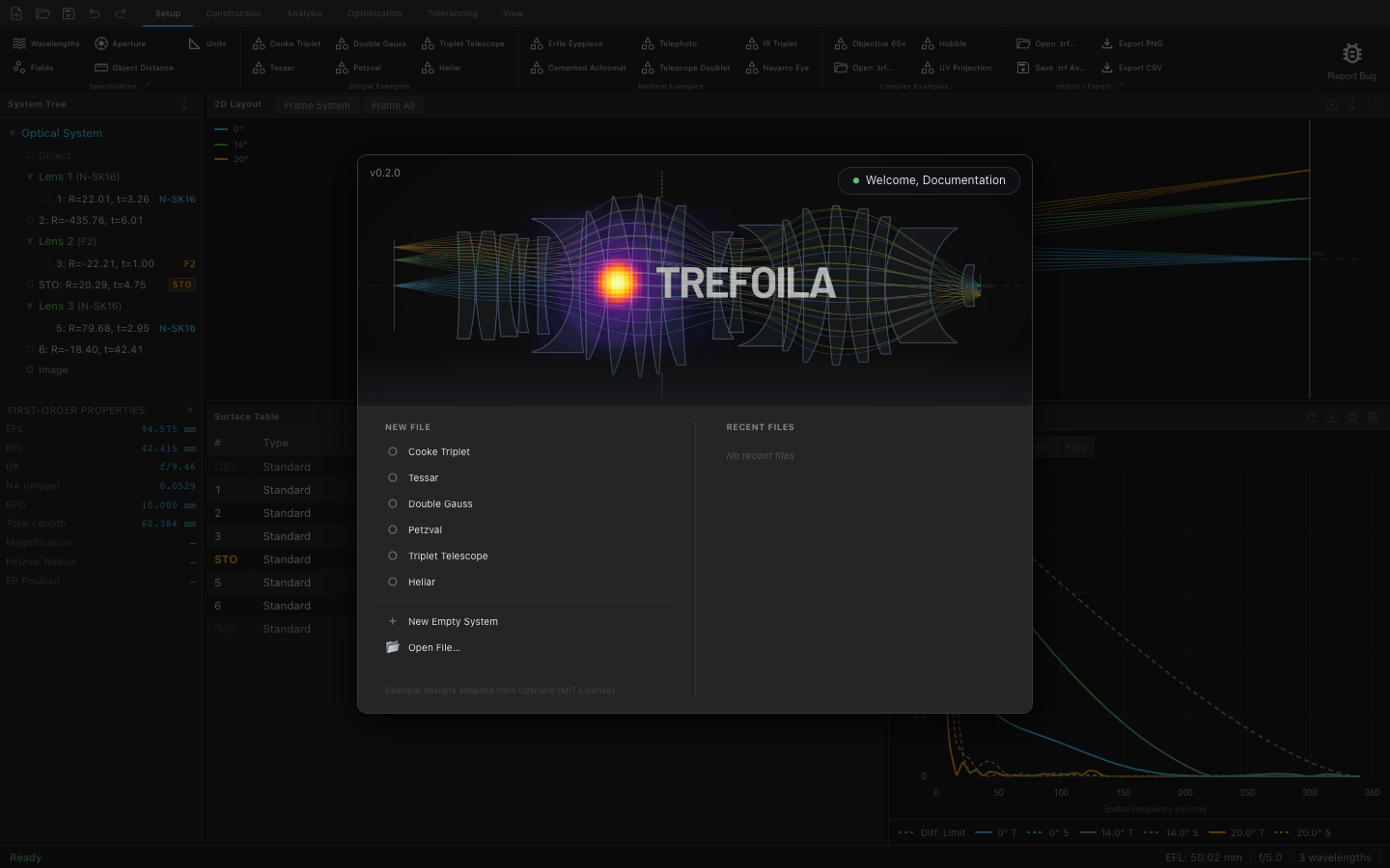
After dismissing the splash, the main window appears with the ribbon toolbar at the top and the panel workspace in the center. You can also reach sample designs any time from the Setup tab.

4. Open a Sample Design

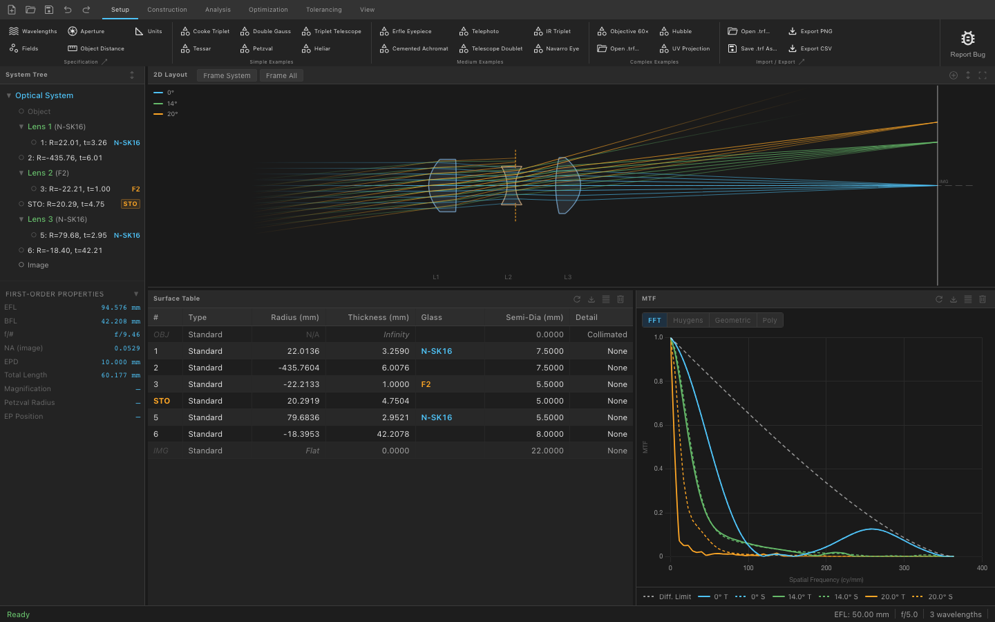
Trefoila ships with fully configured example systems. The Cooke Triplet is a classic photographic lens (f/5, 10 mm entrance pupil) and is a good starting point for exploring the application.

1. Click the Setup tab in the ribbon.
2. In the Samples group, click Cooke Triplet.

After opening, the 2D Layout panel appears automatically, showing the lens cross-section with ray fans traced through the system.

The status bar at the bottom now shows the system's first-order properties: EFL, f/#, and Strehl ratio. These update automatically whenever you change any surface parameter.

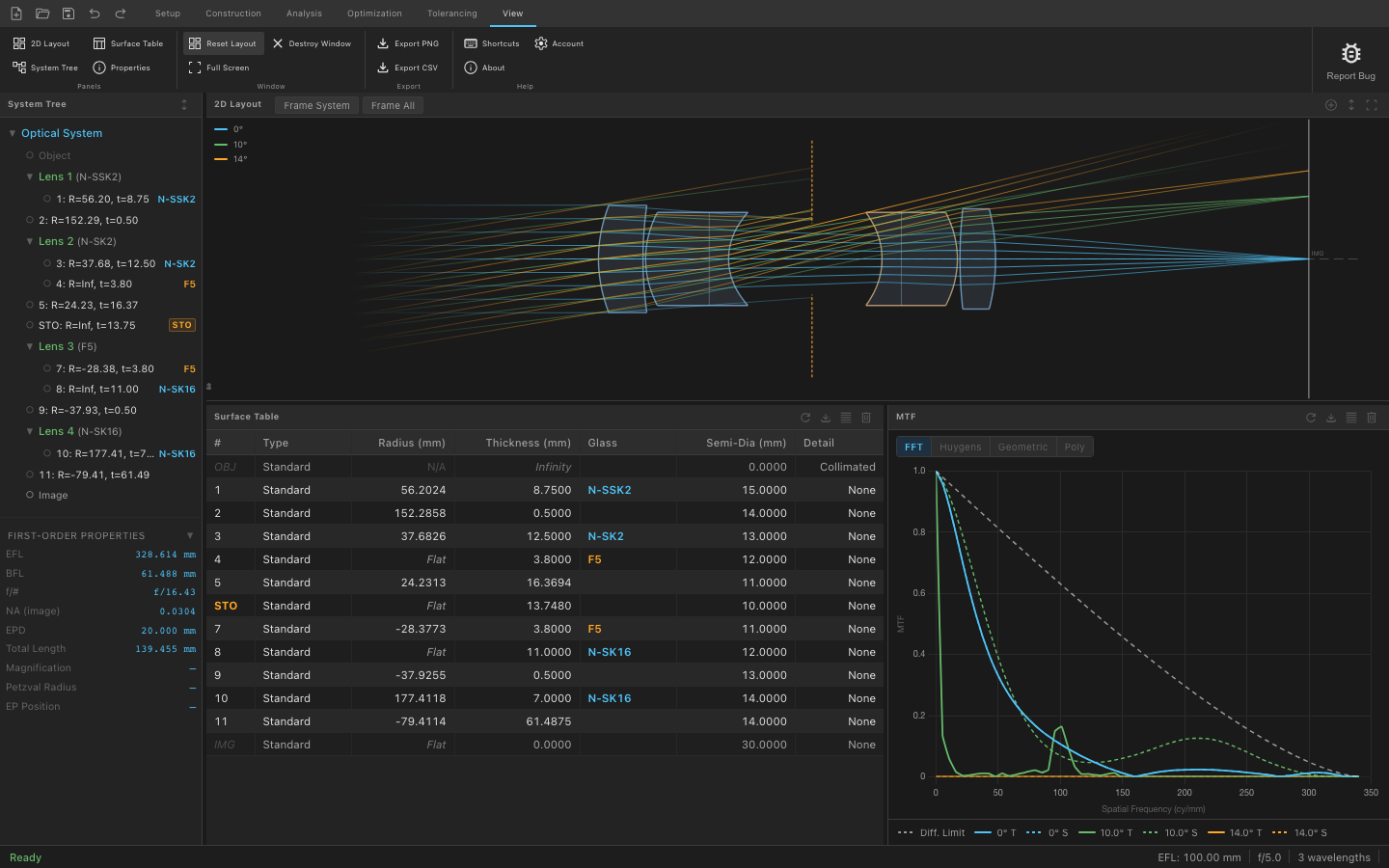
5. Understanding the Interface

The main window has four regions:

Region	Location	Description
Ribbon Toolbar	Top	Six tabs — Setup, Construction, Analysis, Optimization, Tolerancing, View — each grouping related commands
System Tree	Far left (narrow strip)	Hierarchical view of surfaces, wavelengths, fields, and aperture
Panel Workspace	Center / right	Flexible tiled area where analysis panels, the layout, and the surface table live
Status Bar	Bottom	Live EFL, f/#, Strehl ratio, and background task progress

Ribbon Tabs

Tab	What you do here
Setup	Define wavelengths, field points, aperture type and size, and object distance
Construction	Edit the surface table — add/remove surfaces, set radii, thicknesses, glass, and aperture shapes
Analysis	Open analysis panels: spot diagram, ray fan, wavefront, PSF, MTF, distortion, and more
Optimization	Define design variables and merit function operands, then run the optimizer
Tolerancing	Run sensitivity analysis and Monte Carlo simulations to predict yield
View	Control panel layout, zoom the 2D view, and export images or data

Panel Workspace

Panels can be opened from the Analysis ribbon tab, resized by dragging their borders, and tiled side by side. Every panel recomputes automatically when the system changes — there is no manual "update" button.

6. Setting Up a Simple Lens

This section walks through entering a lens from scratch. If you are working with the Cooke Triplet sample, follow along to understand each step — you can inspect the values already entered without changing them.

6.1 Surface Table

Click the Construction tab in the ribbon. The Surface Table panel opens in the workspace.

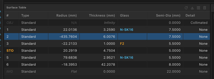
The table always starts with an Object surface (row 0) and ends with an Image surface. Every row in between is a physical optical surface or a gap.

Column	Description
Radius	Radius of curvature in mm. Positive = center of curvature to the right. Inf = flat.
Thickness	Axial distance to the next surface in mm.
Glass	Material name (e.g. N-BK7) or blank for air.
Semi-Diam.	Clear aperture radius in mm. Auto-calculated if left blank.
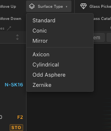
Type	Standard, Conic, Mirror, etc. Most surfaces are Standard.

To add a surface, right-click any row and choose Insert Surface After. To delete a surface, right-click and choose Delete Surface.

Double-click any surface row to open the Surface Properties dialog for full control over that surface.

6.2 Glass

Click directly on any Glass cell in the surface table to open the Glass Picker. You can search by name, filter by catalog (Schott, Ohara, Hoya, and others), or enter a custom index and Abbe number.

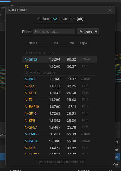
Leave the Glass cell blank to use air (n = 1.000). For mirrors, set Glass to MIRROR — Trefoila handles the sign reversal automatically.

6.3 Fields & Aperture

Click the Setup tab, then click Fields to open the fields dialog. Each field point defines an angle (for infinite-conjugate systems) or an object height (for finite conjugate systems) at which the system is evaluated.

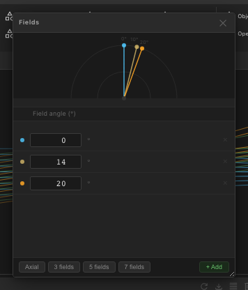
Add field points by clicking Add Field. A typical starting set is three fields: on-axis (0°), 70 % of full field, and full field. Analysis panels color-code results by field point so you can compare them at a glance.

Back in the Setup tab, click Aperture to set the entrance pupil diameter (EPD). You can also specify the aperture as an image-space f-number or numerical aperture depending on your design intent.

7. Running Your First Analysis

Once a system is defined, open analysis panels from the Analysis tab. Each panel is independent and can be open simultaneously.

Spot Diagram

Click Analysis → Spot Diagram. A grid of spot plots appears, one cell per field point. The geometric RMS spot radius is shown below each cell.

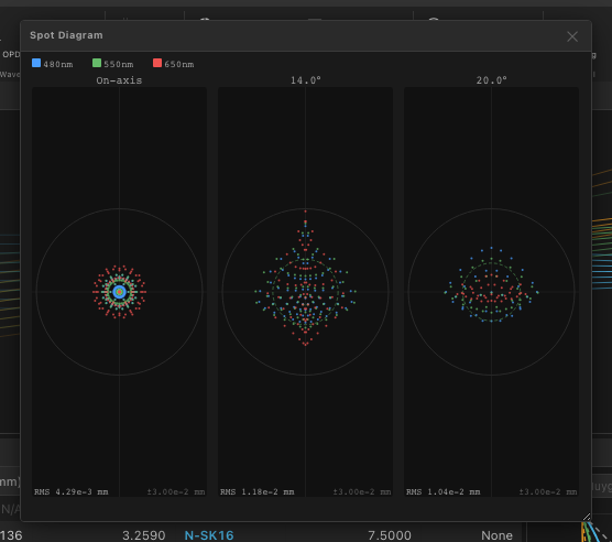
Each wavelength is plotted in a different color. The Airy disk radius is shown as a reference circle when the system is diffraction-limited or near it. Pan and zoom individual cells with the mouse.

Ray Fan

Click Analysis → Ray Fan. The tangential (T) and sagittal (S) fans are shown for each field point. The horizontal axis is normalized pupil coordinate; the vertical axis is transverse aberration in mm.

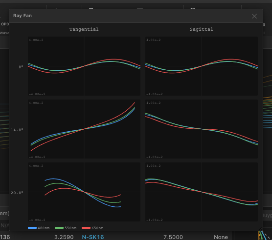
S-shaped curves indicate third-order spherical aberration. Straight sloped lines indicate defocus. Asymmetry between T and S fans indicates astigmatism or coma.

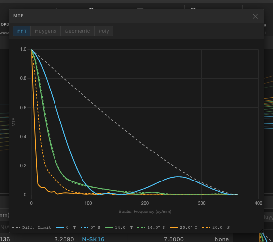
MTF

Click Analysis → MTF. The modulation transfer function is plotted against spatial frequency (cycles/mm at the image plane) for each field point, tangential and sagittal separately.

8. Optimization

Trefoila's optimizer adjusts surface radii, thicknesses, glass indices, and conic constants to minimize a merit function you define. This section walks through the essentials.

1. Click the Optimization tab, then click Optimization Studio to open the combined setup panel.
2. Set variables. In the Variables section, check the radius or thickness of each surface you want the optimizer to change. A blue V badge appears on those cells in the surface table.
3. Define the merit function. The default merit function minimizes RMS wavefront error across all fields and wavelengths, which is a practical starting point for most designs. Add custom operands (focal length, distortion, back focal distance, etc.) from the operand list.

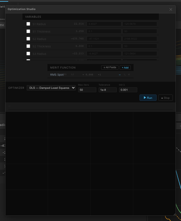
4. Click Run. The merit function value is shown in real time as the optimizer iterates. Analysis panels that are open update live so you can watch the design improve.

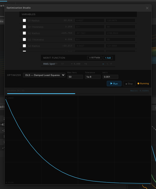
Trefoila offers four algorithms selectable from the optimizer toolbar:

Algorithm	Best for
DLS (Damped Least Squares)	Polishing a near-final design; fast convergence when close to optimum
Nelder-Mead	Non-differentiable merit functions; robust but slow
Differential Evolution	Global search with many variables; good for finding fundamentally better forms
Hybrid DE+DLS	Global search followed by local polish; a solid default for new designs

9. Saving Your Work

Save

Press Ctrl/Cmd+S or click File → Save. Projects are saved in the .trf format — plain JSON text that is fully human-readable and diff-friendly for version control.

Save As

Use Ctrl/Cmd+Shift+S to save to a new filename. This is useful when creating design variants or when working from a sample file you want to keep unmodified.

Export

Use File → Export to share designs. Export options include:

• PNG / SVG — export the 2D layout or any analysis plot as an image
• CSV — export surface data, aberration tables, or MTF data for use in spreadsheets or reports

---

You now have everything you need to explore Trefoila. For detailed documentation on any feature — surface types, advanced apertures, tolerancing, coatings, the file format — see the User Manual.

Trefoila v0.2.0  ·  © 2026 Blake Griffiths  ·  All rights reserved