1. Introduction

Trefoila is a professional lens design application built for optical engineers, researchers, and students. It combines a fast sequential ray-tracing engine with a modern, responsive graphical interface.

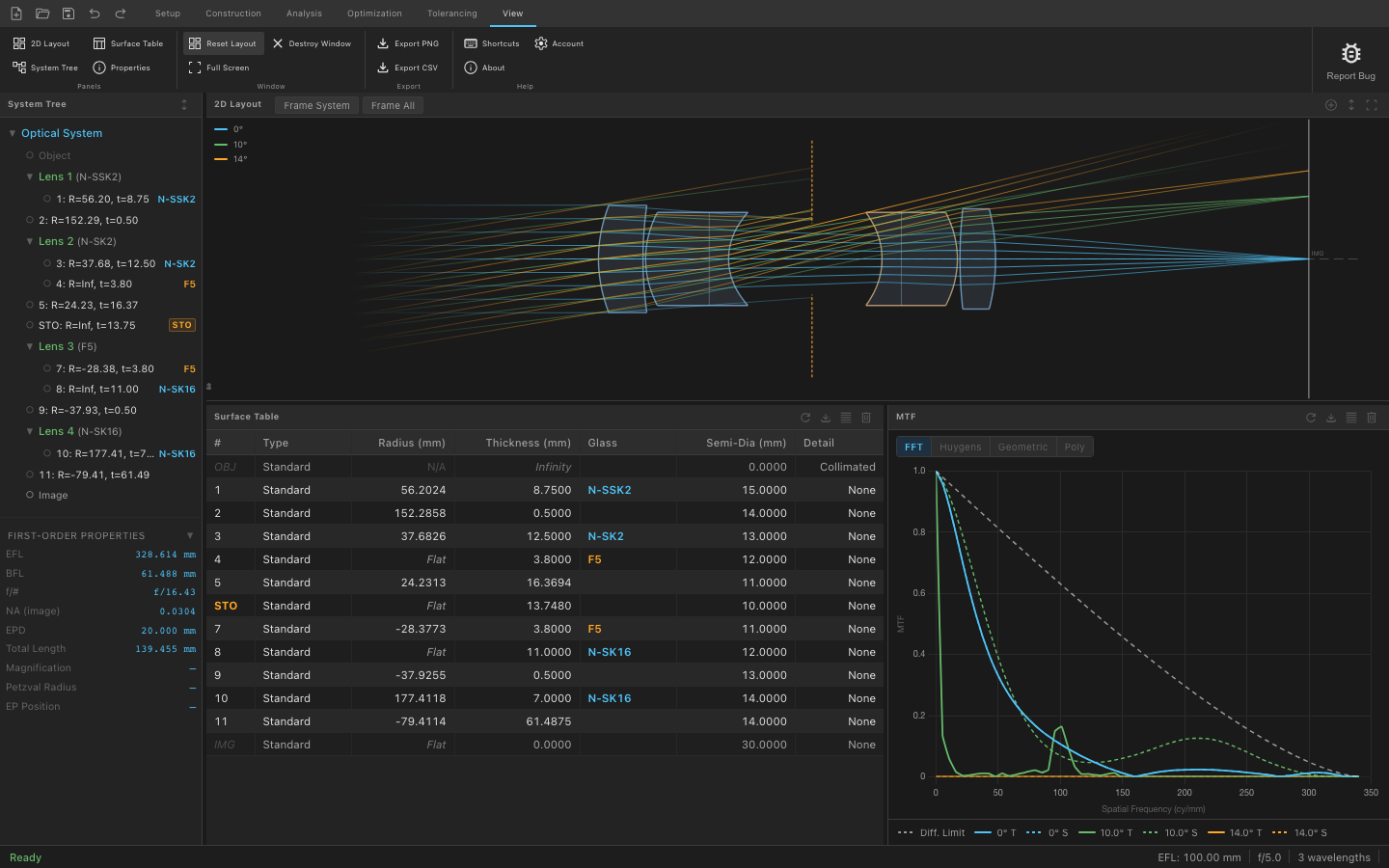
The application is organized around a familiar ribbon toolbar (Setup, Construction, Analysis, Optimization, Tolerancing, View) and a flexible panel workspace where you can tile any combination of plots and tables side by side. Every analysis panel updates automatically whenever the system changes.

Key Capabilities

• Sequential ray tracing powered by a native Rust engine
• Surface types: Standard (spherical), Conic/Asphere, Mirror, Zernike Freeform, Odd Asphere, Cylindrical/Toroidal, Axicon
• Glass catalog (Schott, Ohara, Hoya, Thorlabs, and custom glasses)
• Multilayer optical coatings with R(λ) / T(λ) curves
• Full wavefront analysis: OPD maps, Zernike decomposition (Noll / Fringe / Standard), Strehl ratio
• MTF: FFT, Huygens, Polychromatic, Geometric, Through-Focus, and MTF at a user frequency
• PSF: FFT and Huygens, linear and log10 scale, through-focus sweep
• Seidel third-order aberrations, chromatic focal shift, longitudinal and lateral CA
• Encircled and ensquared energy, vignetting, distortion, ghost analysis
• Optimization: DLS, Nelder-Mead, Differential Evolution, hybrid DE+DLS
• Tolerancing: sensitivity tables, inverse sensitivity, Monte Carlo, RSS budget breakdown
• Finite conjugate (microscope, projection) systems
• Solves and pickups for automatic parameter constraints
• Import/export: .trf native format

2. Interface Overview

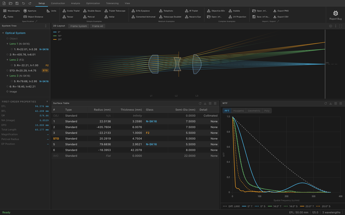
The main window is divided into four regions:

Region	Location	Description
Ribbon	Top	Tabbed toolbar with all commands organized by workflow phase
System Tree	Far left (narrow)	Hierarchical view of the optical system: surfaces, wavelengths, fields, aperture
Panel Workspace	Center / right	Flexible tiled area for layout, analysis plots, and the surface table
Status Bar	Bottom	EFL, f/#, Strehl ratio, last action, and background task progress

2.1 Ribbon Toolbar

The ribbon contains six tabs. Click any tab to reveal its group of commands. Buttons with a small arrow open a dropdown with sub-options.

The Quick Access Bar (left side of the ribbon, always visible) provides one-click access to the most common file operations:

Button	Shortcut	Action
New System	Ctrl/Cmd+N	Create a blank optical system
Open Project	Ctrl/Cmd+O	Open a .trf file
Save	Ctrl/Cmd+S	Save the current project
Undo	Ctrl/Cmd+Z	Undo last edit
Redo	Ctrl/Cmd+Shift+Z	Redo last undone edit

2.2 Panel System

The workspace is a split container. You can tile any number of analysis panels side by side or stacked vertically. Each panel has a title bar with a close button.

Opening a panel: click the corresponding button in the ribbon, or use the View tab → Panels group. If a panel is already open it will be focused; otherwise it opens in the next available slot.

Closing a panel: click the × on the panel title bar, or use View → Destroy Window (then click the panel you want to remove).

Reset Layout: View → Reset Layout restores the default four-panel arrangement (System Tree · 2D Layout · Surface Table · MTF).

2.3 Status Bar

The status bar at the bottom of the window shows live system metrics that update after every edit: EFL (effective focal length), f/#, Strehl ratio, and the most recent action name. During long computations (optimization, Monte Carlo) a progress indicator appears on the right.

3. Getting Started

3.1 New / Open / Save

New system: press Ctrl/Cmd+N or click the note_add icon in the quick-access bar. A blank system is created with an object surface, one standard refractive surface, and an image surface.

Opening a project: press Ctrl/Cmd+O or click Open .trf… in the Setup tab → Import/Export group. Navigate to a .trf file and click Open. All surfaces, wavelengths, fields, aperture settings, coatings, and solves are restored.

Saving: Ctrl/Cmd+S saves to the current file. Use Save .trf As… in the ribbon to save to a new location.

3.2 Sample Designs

Over a dozen fully configured example designs are included. Access them from Setup → Simple / Medium / Complex Examples:

Group	Designs
Simple	Cooke Triplet, Tessar, Double Gauss, Petzval, Triplet Telescope, Heliar
Medium	Erfle Eyepiece, Cemented Achromat, Telephoto, Telescope Doublet, IR Triplet, Navarro Eye
Complex	Objective 60×, Hubble, UV Projection

4. Setup Tab

The Setup tab is where you define the fundamental parameters of your optical system before designing surfaces.

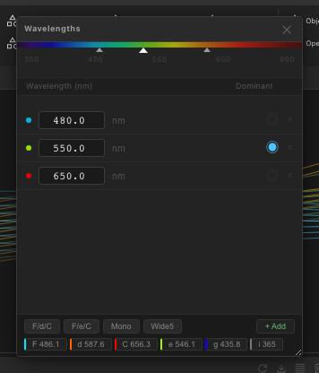
4.1 Wavelengths

Click Wavelengths in the Specification group to open the Wavelengths dialog. You can define up to several wavelengths in microns. One wavelength is designated the primary wavelength, which is used as the default for monochromatic analyses. Color-coded markers correspond to the wavelength colors shown in spot diagrams, ray fans, and MTF plots.

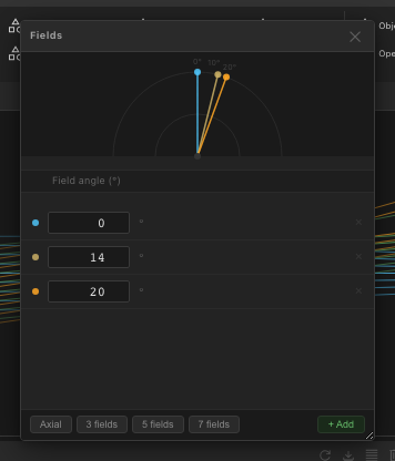
4.2 Fields

Click Fields to define the angular or spatial field points used in analysis. Each field is a half-angle (degrees) for infinite-conjugate systems, or an object height (mm) for finite-conjugate systems. Each field gets a unique color used consistently across all analysis panels.

The field type is set by your Object Distance setting: if the object is at infinity, fields are angles; if the object is at a finite distance, fields are object heights.

4.3 Aperture

The aperture setting controls how the entrance pupil size is specified. Click the Aperture dropdown button to choose the aperture type, then click the button itself to enter the value.

Type	Description
Entrance Pupil Diameter (EPD)	Directly sets the entrance pupil diameter in system units. Most common choice for camera and telescope lenses.
Image-Space f/#	Sets the f-number (focal length ÷ entrance pupil diameter). Use when you know the desired f-stop.
Object-Space NA	Sets the numerical aperture on the object side. Common for microscope objectives.
Float by Stop	The aperture is determined by the physical semi-diameter of the stop surface. Useful when the stop size is the primary constraint.

4.4 Object Distance

Click Object Distance to set the distance from the object plane to the first surface. Enter a large value (e.g., 1e+18) for an effectively infinite conjugate, or a finite value in system units for close-focus or microscope systems. Changing from infinite to finite conjugate switches field specification from angles to object heights.

4.5 Units

Click Units to set the system units: mm (default), cm, m, or inches. All radius, thickness, and semi-diameter values in the surface table are displayed in these units. Internal computations and glass catalog data are always in mm; the unit setting only affects display.

5. Construction Tab

The Construction tab is where you build the physical optical system: add and configure surfaces, assign glass materials, add coatings, and set up advanced parameters like solves and pickups.

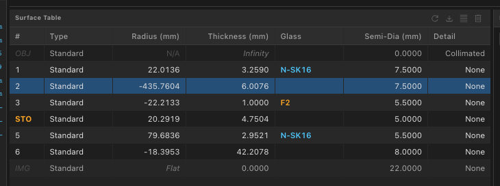
5.1 Surface Table

The Surface Table panel is the central editing interface for the optical prescription. It displays one row per surface with the following columns:

Column	Description
#	Surface index. Surface 0 is always the object; the last surface is always the image.
Type	Surface type (Standard, Conic, Mirror, etc.)
Radius	Radius of curvature. Positive = center of curvature to the right. Inf = flat.
Thickness	Axial distance to the next surface. Type SOL or SOLVE to open the Solve dialog.
Glass	Material after this surface. Click to open the glass picker. Leave blank for air.
Semi-Dia	Semi-diameter (half clear aperture). Auto-computed from ray trace if left blank.
Detail	Shows conic constant, coating name, solve type, or aperture shape, depending on what is set.

Click any cell to edit it. Click a row to select that surface; the selected row is highlighted and used as context for ribbon operations (Delete, Duplicate, Move, Set Stop, etc.).

Right-click on any row to access a context menu with Insert, Delete, Duplicate, Move Up, Move Down, and Set as Stop.

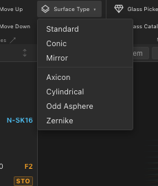
5.2 Surface Types

Click Add Surface (large button) in the Construction tab to insert a new surface after the selected one. The dropdown lists all available types:

Type	Description
Standard (Spherical)	A sphere defined by radius of curvature. The workhorse surface for most designs.
Conic / Asphere	Spherical + conic constant (k) + even aspheric polynomial terms A₂, A₄, A₆…. Paraboloids (k=−1), hyperboloids (k<−1), ellipsoids (−1<k<0), oblate spheroids (k>0).
Mirror	Reflective surface. Thickness after a mirror should be negative to reverse the propagation direction. Same sag equation as Conic/Asphere.
Zernike Freeform	Base sphere plus a Zernike polynomial departure map. Useful for freeform optics and wavefront correction elements.
Odd Asphere	Aspheric polynomial including odd powers (A₁r, A₃r³, …). Used for axicons and near-diffractive elements.
Cylindrical / Toroidal	Surface with curvature in only one meridian. Used for cylindrical lenses and anamorphic optics.
Axicon	Conical surface producing a Bessel beam. Defined by its cone half-angle.

To change the type of an existing surface, select the surface and use the Surface Type dropdown in the ribbon. Parameters unique to the new type will be initialized to their defaults; radius and thickness are preserved.

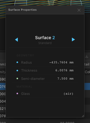
Surface type-specific parameters (conic constant, aspheric coefficients, Zernike terms, grating period, etc.) are edited via the Surface Properties button in the Construction tab → Advanced group.

5.3 Materials & Glass

Glass is assigned per surface: it defines the refractive material for rays traveling from that surface to the next. An empty glass cell means air (n=1).

Glass Picker: Select a surface and click Glass Picker (or double-click the Glass cell). A searchable dialog lists all glasses from the loaded catalogs, with Abbe number and nd value displayed. Type to filter by name, nd, or Vd.

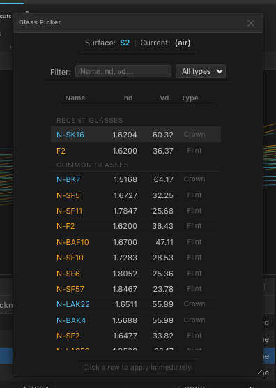
Glass Catalog panel: Open with Glass Catalog button or via the dialog launcher arrow in the Materials group. Shows the full catalog in a table with sortable nd, Vd, density, and transmission columns. You can browse and compare glasses before assigning them.

Custom Glasses: Click Custom Glasses to define your own glass using a Sellmeier equation or direct nd/Vd entry. Custom glasses are saved with the project.

5.4 Coatings

Optical coatings affect both the appearance of the layout and (optionally) the throughput calculation. A coating can be assigned to any surface.

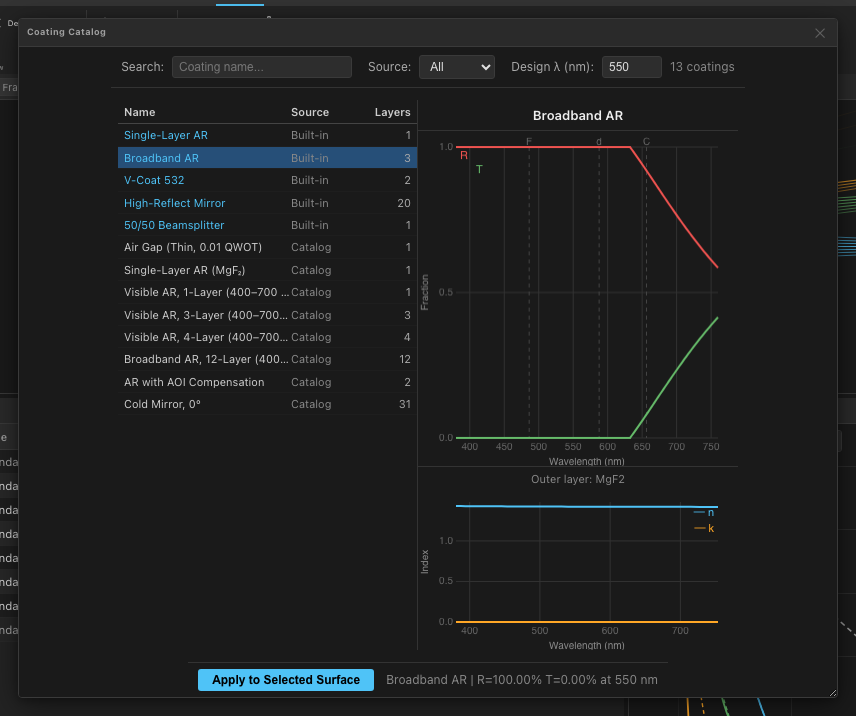
Coating Picker: Select a surface and click Coating Picker. Choose from preset coatings (AR broadband, V-coat, HR mirror, etc.) or any coating in the catalog.

Coating Catalog: A panel showing all available coatings with R(λ) and T(λ) curves plotted interactively. Click any row to preview the spectral response.

Custom Coating: Build a multilayer coating by specifying layer materials and thicknesses. The panel shows a live R(λ)/T(λ) preview as you adjust layers, using a transfer matrix thin-film model.

5.5 Advanced Construction Features

Solves

A solve is a constraint that automatically adjusts a surface parameter to satisfy a condition. Click Solves in the Advanced group (or type SOL in the Thickness cell) to open the Solve dialog for the selected surface. Available solve types include:

• Marginal Ray Height — adjusts thickness so the marginal ray hits a specified height at the next surface
• Chief Ray Angle — adjusts thickness to achieve a specified chief ray angle
• Edge Thickness — adjusts thickness to maintain a minimum edge thickness
• Pick Up — links this parameter to another surface's parameter (see Pickups)

Pickups

A pickup links a parameter on one surface to a parameter on another, with an optional scale and offset. Click Pickups to open the pickup editor. Common use: make a lens' back radius the negative of its front radius (for an equiconvex lens), or couple thicknesses across multiple configurations.

Quick Focus

Click Quick Focus to automatically set the image distance (thickness of the last optical surface to the image plane) to place the paraxial focus exactly on the image surface. This is equivalent to a marginal ray height = 0 solve on the last thickness.

5.6 Aperture Shapes

Every surface can have a physical aperture shape assigned, which clips rays that fall outside the aperture boundary. Click Aperture Shape in the Apertures group and select the desired shape:

• Circular — standard circular clear aperture, defined by the semi-diameter
• Rectangular — defined by half-width and half-height
• Elliptical — defined by semi-axes in X and Y
• Annular (Obscured) — circular with a central obstruction (inner radius). Used for mirrors with a secondary obstruction (e.g., Cassegrain telescopes).
• Polygon (Hex, etc.) — arbitrary polygon defined by vertex coordinates. Used for hexagonal mirrors, rectangular prisms, etc.

After selecting the shape type, the dialog for that shape opens so you can enter dimensions. The shape is shown in the Detail column of the Surface Table and is respected by all ray trace operations.

6. 2D Layout

The 2D Layout panel shows a cross-sectional view of the optical system with lens element shapes, ray traces for all defined fields, and labeled key planes (entrance pupil, exit pupil, focal planes).

Navigation:

• Scroll wheel / pinch — zoom in/out centered on the cursor position
• Click and drag — pan the view
• The view automatically fits the system when a new design is loaded

What is shown:

• Lens elements are drawn with their correct cross-sectional profile shapes (meniscus, biconvex, plano-concave, etc.)
• Mirror surfaces are shown as reflective elements with the correct curvature
• Ray fans are color-coded to match the field colors set in the Fields dialog
• For infinite-conjugate systems, ray tails on the left side fade out with decreasing opacity to indicate the incoming collimated beam
• The object plane is shown as a dashed vertical line when the system has a finite object distance ≥ 1 mm
• The image plane is shown as a solid vertical line on the right

7. Analysis Tab

The Analysis tab provides access to every optical analysis tool. All panels update automatically when the system changes; press F9 or Refresh All to force an immediate update of every open panel.

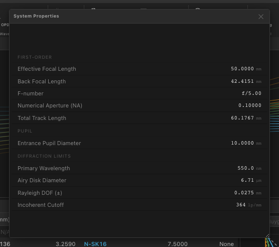
7.1 System Properties

Open with Analysis → Paraxial → Properties, or View → Properties. This panel displays first-order optical properties computed from a paraxial ray trace:

Property	Description
EFL	Effective focal length (image-space, in system units)
BFL	Back focal length (vertex of last surface to rear focal point)
f/#	F-number = EFL / entrance pupil diameter
Working f/#	Effective f-number accounting for conjugate ratio and vignetting
NA (image)	Image-space numerical aperture
Entrance Pupil Dia.	Entrance pupil diameter at the object-space pupil location
Entrance Pupil Pos.	Axial position of entrance pupil from the first surface vertex
Magnification	Paraxial lateral magnification (finite conjugate only)
Total Length	Axial distance from first surface to image surface
Image Distance	Distance from last optical surface vertex to image plane
Petzval Radius	Petzval field curvature radius
Surfaces / Elements / Wavelengths / Fields	System structure summary

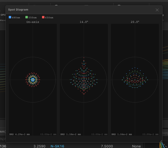
7.2 Spot Diagram

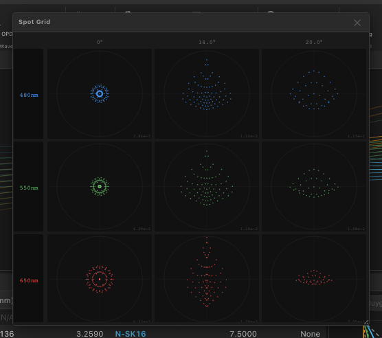
Open via Analysis → Ray Distribution → Spot Diagram. Also available: Spot Grid (a grid of spot diagrams, one per field, for a compact multi-field view).

The spot diagram plots the X-Y intercepts of a fan of rays at the image plane, color-coded by field. The spread of the spot is a direct measure of geometric aberration. A perfect, diffraction-limited system would show all rays within an Airy disk radius.

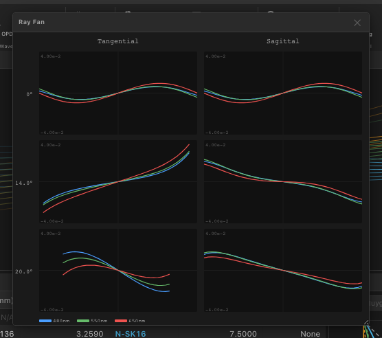
7.3 Ray Fan

Open via Analysis → Ray Distribution → Ray Fan. Three modes are available from the dropdown: Tangential Fan, Sagittal Fan, or Both (T + S) (default). The mode can also be changed using the Show dropdown inside the panel.

The tangential fan plots the Y-component of transverse ray error (EY) vs. normalized pupil coordinate Y for each field and wavelength. The sagittal fan plots the X-component (EX) vs. pupil coordinate X. Deviations from a flat line indicate aberrations:

• Straight tilted line — defocus (longitudinal error)
• S-curve — spherical aberration
• Offset between fields — coma
• Difference between T and S fans — astigmatism
• Wavelength spread — chromatic aberration

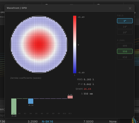
7.4 Wavefront / OPD

Open via Analysis → Wavefront → Wavefront / OPD. The panel has two parts:

• Left: OPD Map — a 2D color image showing the optical path difference across the exit pupil, in waves. The color scale runs from blue (negative OPD) to red (positive OPD). A perfectly corrected system would show a uniform color (zero OPD).
• Right: Zernike Coefficients Table — the OPD map decomposed into Zernike polynomial terms. Rows show term index, name (e.g., Z4 = Defocus, Z8 = Primary Coma), and coefficient value in waves.

Use the Field dropdown to select which field point to analyze. Use the Zernike dropdown to choose the ordering convention: Noll (most common), Fringe, or Standard (ANSI).

The RMS wavefront error (W_rms) is displayed in the header bar, in waves.

7.5 Strehl Ratio

Click Analysis → Wavefront → Strehl Ratio to compute the Strehl ratio for each field point. The Strehl ratio is computed using the Maréchal approximation:

S = exp(−(2π · W_rms)²)

A result of 1.0 is diffraction-limited. Values above 0.8 (the Maréchal criterion) are considered diffraction-limited in practice. If the RMS wavefront error exceeds 20λ the result is shown as N/A.

Results are displayed in a popup dialog listing each field angle and its Strehl value.

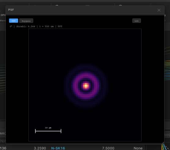
7.6 PSF (Point Spread Function)

Open via Analysis → PSF/MTF → PSF. Two computation methods are available:

• FFT PSF — computes the PSF via a fast Fourier transform of the pupil function (OPD). Very fast; assumes a uniform pupil with no vignetting.
• Huygens PSF — computes the PSF by summing Huygens wavelets from sampled pupil points. Slower but accounts for vignetting and pupil aberrations more accurately.

Use the Field dropdown to select the field point. Use the Scale dropdown to toggle between Linear and Log10 intensity scales. Log scale is useful for seeing diffraction rings that are invisible at linear scale.

Additional options from the dropdown:

• Through-Focus PSF — sweeps the image plane through focus and plots Strehl ratio vs. defocus position as a line graph, useful for visualizing depth-of-field behavior.
• Depth of Focus — computes and displays the axial depth over which the Strehl ratio stays above a threshold (default 0.8).

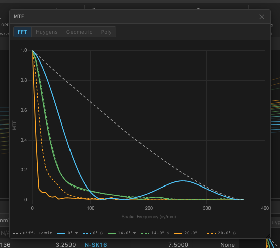
7.7 MTF (Modulation Transfer Function)

Open via Analysis → PSF/MTF → MTF. The panel plots MTF (contrast, 0–1) vs. spatial frequency (cycles/mm) for all fields and both tangential and sagittal orientations. A dashed line shows the diffraction limit for comparison.

Four computation methods are available from the Method dropdown at the top of the panel:

Method	Description
FFT MTF	Derived from the FFT of the pupil function. Fast; most commonly used.
Polychromatic MTF	Averages the MTF across all defined wavelengths, weighted by relative illumination. Gives a realistic polychromatic performance estimate.
Geometric MTF	Computed from the spot diagram distribution. Fast but less accurate for near-diffraction-limited systems.
Huygens MTF	Derived from the Huygens PSF. Most accurate but slowest; recommended for precision analysis.

Additional options from the ribbon dropdown:

• MTF at Frequency… — opens a panel showing a bar chart of MTF values at a specific user-specified frequency, for all fields. Useful for comparing designs against a sensor's Nyquist frequency.
• Through-Focus MTF — plots MTF at a fixed frequency as a function of defocus position.

7.8 Encircled / Ensquared Energy

Open via Analysis → Energy & Ghosts → Encircled Energy. This panel plots the fraction of total PSF energy contained within a circle (encircled) or a square (ensquared) of increasing radius, for each field point.

Switch between modes using the dropdown: Encircled Energy (Circular) computes within a circular aperture; Ensquared Energy (Square) computes within a square aperture (relevant when the detector has square pixels).

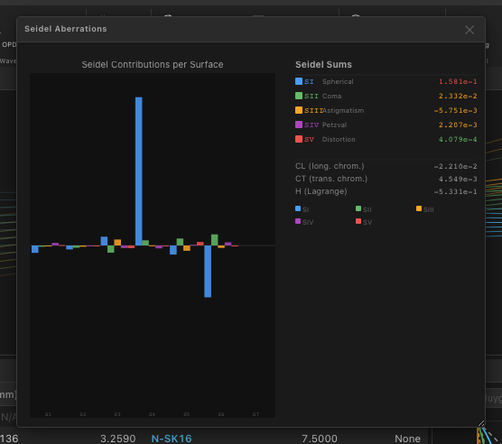
7.9 Seidel Aberrations

Open via Analysis → Aberrations → Seidel. This panel displays a bar chart and table of the five Seidel (third-order) aberration coefficients:

• W040 — Spherical Aberration (SI)
• W131 — Coma (SII)
• W222 — Astigmatism (SIII)
• W220 — Field Curvature (SIV)
• W311 — Distortion (SV)

Values are shown per surface and as totals, so you can see which surfaces contribute most to each aberration type.

7.10 Chromatic Aberrations

Open via Analysis → Aberrations → Chromatic. Four sub-analyses are available from the dropdown:

Mode	Description
Chromatic Focal Shift	Plots the longitudinal focus position as a function of wavelength. A flat line = no axial color; a large spread = high axial chromatic aberration.
Longitudinal CA (Axial Color)	The difference in focus position between the short and long wavelengths, as a function of field.
Lateral CA (Transverse Color)	The difference in image height between wavelengths at the image plane. Appears as color fringing at the edge of the field.
Secondary Spectrum	Plots the residual chromatic focal shift after paraxial achromatization, as a function of wavelength.

7.11 Vignetting

Open via Analysis → Ray Distribution → Vignetting. This panel shows how much of the entrance pupil is vignetted (blocked by physical apertures) as a function of field angle. The companion Relative Illumination plot shows the resulting irradiance falloff at the image plane relative to the on-axis field.

7.12 Distortion

Open via Analysis → Ray Distribution → Distortion. Plots the percentage distortion as a function of field angle. Barrel distortion is negative (image smaller than ideal); pincushion distortion is positive.

7.13 Aberration Summary

Open via Analysis → Aberrations → Summary. This panel aggregates three analyses into a single scrollable view:

1. Seidel Aberrations table — the five Seidel coefficients
2. Zernike Coefficients table — Zernike decomposition of the wavefront for the current field, in waves
3. RMS Spot Radius by Field — spot size table listing RMS radius (mm) for each field and each wavelength

This is a useful single-panel snapshot for reporting or comparing designs.

7.14 Through-Focus Analysis

Access through-focus tools from the PSF and MTF dropdowns:

• Through-Focus PSF — sweeps the image plane axially and displays the PSF at each defocus position as a tiled grid or animation. Reveals the shape of the out-of-focus blur (axial astigmatism shows as a rotating ellipse, spherical aberration shows as an expanding ring).
• Through-Focus MTF — plots MTF at a fixed frequency (set in the panel) as a function of defocus position. The peak of this curve is the best focus position.
• Depth of Focus — a summary popup showing the ±defocus range over which the Strehl ratio stays above 0.8, and the corresponding f-number and wavelength.

7.15 Ghost Analysis

Accessible from Analysis → Energy & Ghosts → Ghost. Ghost analysis identifies spurious images formed by double reflections between lens surfaces. This feature is in development and will be enabled in a future update.

8. Optimization Tab

The Optimization tab provides lens design optimization: you define which surface parameters are free to vary (variables), what the optimizer tries to minimize (merit function), and which algorithm to use.

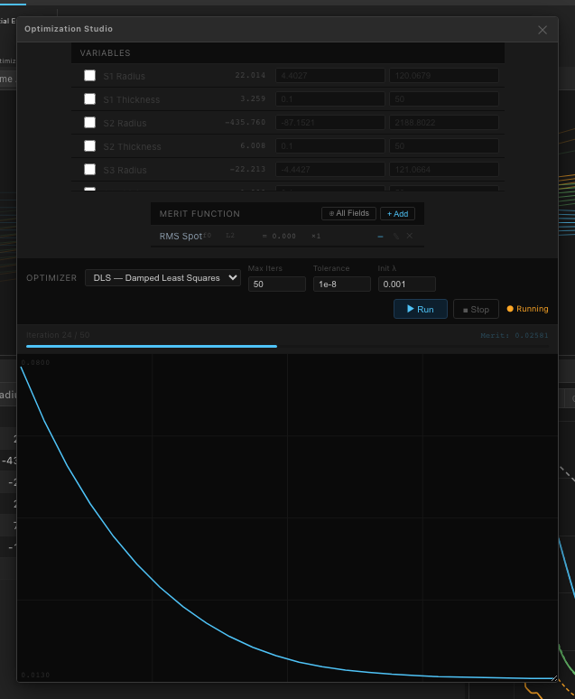
8.1 Optimization Studio

The quickest way to set up and run an optimization is the Optimization Studio: a single floating window containing the Variables editor, Merit Function builder, and Optimizer controls all in one place. Open it from Optimization → Optimization Studio.

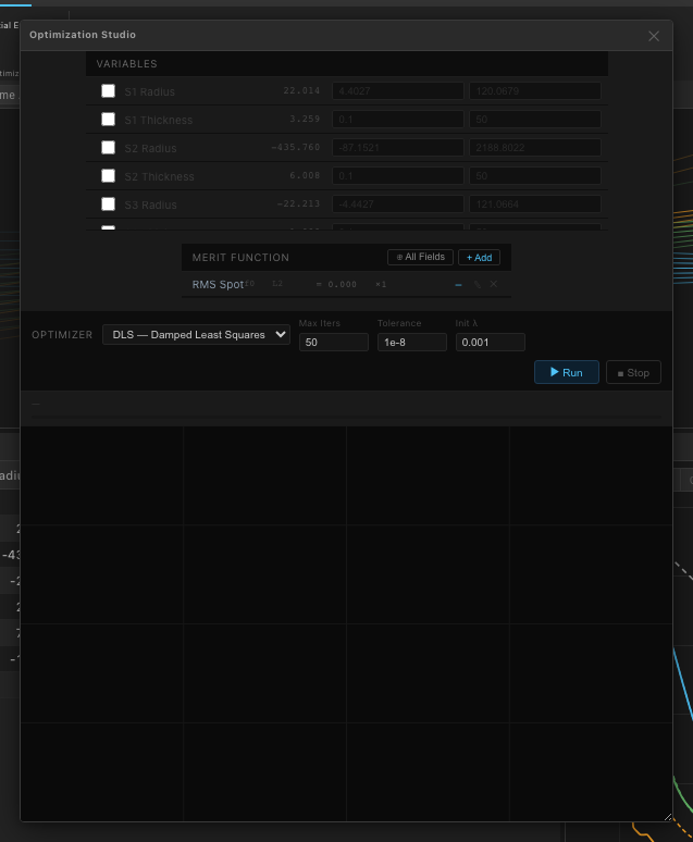
8.2 Variables

Open via Optimization → Variables. Variables are the surface parameters that the optimizer is allowed to change. For each variable you specify:

• Surface index — which surface
• Parameter — Radius, Thickness, Conic, or aspheric coefficient (A4, A6, …)
• Min / Max bounds — the allowed range for this variable
• Current value — shown live, updates as the optimizer runs

Typical starting point for a triplet: radii of surfaces 1–6 as variables, with the thicknesses fixed, and the image distance as a solve.

8.3 Merit Function

Open via Optimization → Merit Function. The merit function is a scalar value that the optimizer minimizes. It is the weighted sum of operands, where each operand is a measurable property of the system. Available operand types include:

Operand	Description
RMS Spot Size	RMS radius of the spot diagram at a given field and wavelength. The most common primary operand.
Effective Focal Length	Penalizes deviation of EFL from a target value. Use to hold EFL constant during optimization.
F-Number	Penalizes deviation of f/# from a target.
Thickness Constraint	Penalizes a thickness going below a minimum value (center or edge). Use to prevent physically impossible thin elements.

Each operand has a weight (default 1.0) and a target value. The total merit function value is:

MF = Σ weight_i · (actual_i − target_i)²

8.4 Optimizers

Four optimization algorithms are available:

Local Optimization

• DLS (Damped Least Squares) — gradient-based local refinement. Fast and effective once you are near a good solution. The classic lens design algorithm. Open from the Local Optimization group or from the Optimization Studio.
• Nelder-Mead — derivative-free downhill simplex method. Useful when the merit function is noisy or non-smooth.

Global Optimization

• Differential Evolution (DE) — evolutionary algorithm that maintains a population of candidate designs. Good at escaping local minima and finding globally better forms from scratch.
• Hybrid (DE + DLS) — runs Differential Evolution to find a promising region, then switches to DLS for local convergence. A good default for starting a new design.

To stop any optimizer, click Stop in the Control group or press the Stop button inside the Optimization Studio.

9. Tolerancing Tab

The Tolerancing tab provides manufacturing tolerance analysis: how much does optical performance degrade when lens parameters deviate from their nominal values within specified manufacturing tolerances?

9.1 Tolerance Studio

The Tolerance Studio is the central tolerancing interface — a single window combining the tolerance table, sensitivity analysis, and Monte Carlo simulation. Open it from Tolerancing → Tolerance Studio.

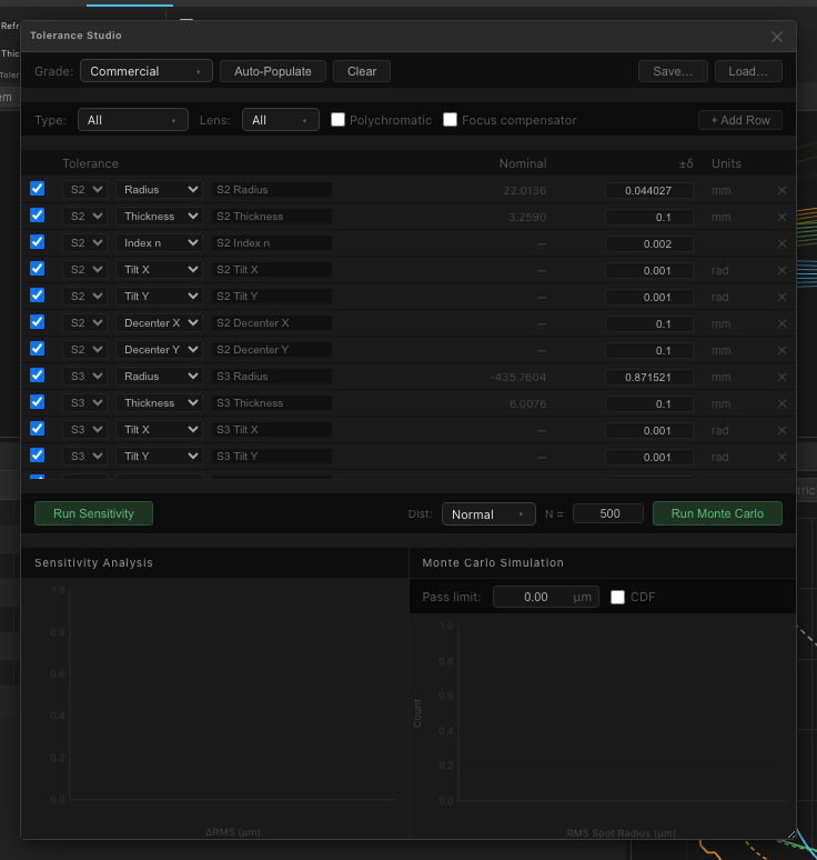
9.2 Sensitivity Analysis

Open via Tolerancing → Windows → Sensitivity. Sensitivity analysis perturbs each tolerance parameter by ±its tolerance value and reports the resulting change in merit function (typically RMS spot size). The output is a table sorted by sensitivity (highest impact first).

Tolerance grades define the default tolerance magnitudes. Three presets are provided:

Grade	Radius (fraction)	Thickness (mm)	Refractive Index (Δn)
Commercial	±0.2%	±0.10	±0.002
Precision	±0.1%	±0.05	±0.001
High Precision	±0.05%	±0.02	±0.0005

You can also edit individual tolerance values in the tolerance table.

9.3 Monte Carlo Simulation

Open via Tolerancing → Windows → Monte Carlo. Monte Carlo simulation generates thousands of random lens realizations where each tolerance parameter is drawn from its probability distribution (uniform or Gaussian within tolerance bounds). The merit function is evaluated for each realization, building a statistical picture of expected performance in production.

The output shows:

• A histogram of merit function values across all MC trials
• Mean, standard deviation, and percentile statistics (P50, P90, P95)
• Worst-case realizations

Set the number of Monte Carlo trials using the spin box (typically 200–1000). More trials give better statistics but take longer.

9.4 Tolerance Types

The following parameter types can be toleranced. Use the Tolerance Types group buttons in the ribbon to filter the tolerance table to show only that type:

Type	Description
Radius	Tolerance on the radius of curvature of each surface. Applied as a fractional deviation (e.g., ±0.1%).
Thickness	Tolerance on the center thickness of each element, and on air gaps. Applied as an absolute deviation in mm.
Tilt	Tolerance on the tip/tilt of each element (degrees). Models lens element wedge and mount-induced tilt.
Decenter	Tolerance on the transverse displacement of each element (mm). Models lens element decentering in its mount.
Refractive Index	Tolerance on the refractive index of each glass (Δn). Models melt-to-melt glass variation.

9.5 Advanced Tolerancing

Inverse Sensitivity: Given a target performance budget (e.g., "the total RSS RMS spot size growth must be ≤ 5 µm"), back-calculate the per-tolerance allocations that achieve this. Open via Tolerancing → Advanced → Inverse Sensitivity.

Compensator: A focus compensator can be enabled, allowing the back focal distance to be re-optimized after each perturbation (modeling refocusing in the final assembly). Enable it via Tolerancing → Advanced → Compensator.

Budget: Shows the RSS (root-sum-square) contribution breakdown: which tolerances contribute most to the total performance degradation. Open via Tolerancing → Advanced → Budget.

10. View Tab

The View tab manages the panel layout and provides window management tools.

Button	Description
2D Layout	Open or focus the 2D Layout panel
Surface Table	Open or focus the Surface Table panel
System Tree	Open or focus the System Tree panel (hierarchical system view)
Properties	Open or focus the first-order Properties panel
Reset Layout	Restore the default four-panel workspace layout
Full Screen	Toggle full-screen mode (F11)
Destroy Window	Enter "destroy mode" — next panel you click will be closed

10.1 Export

Any analysis panel can be exported independently:

• Export PNG — click View → Export → Export PNG to enter export mode, then click the panel you want to save. A resolution dialog appears (1×, 2×, 4× screen resolution, or custom up to 16×). The file is saved as a PNG image. The 4× option is suitable for publication-quality figures.
• Export CSV — click Export CSV, then click a panel. The underlying numeric data (spot coordinates, MTF values, etc.) is exported as a comma-separated file for further processing in Excel, Python, MATLAB, etc.

Both export modes are also accessible from Setup → Import/Export → Export Image… dropdown.

11. Keyboard Shortcuts

Shortcut	Action
Ctrl/Cmd+N	New system
Ctrl/Cmd+O	Open project
Ctrl/Cmd+S	Save project
Ctrl/Cmd+Z	Undo
Ctrl/Cmd+Shift+Z	Redo
F9	Refresh all analysis panels
F11	Toggle full screen
Escape	Cancel export / destroy mode; close Optimization Studio
Delete	Delete selected surface
Ctrl/Cmd+D	Duplicate selected surface

12. File Format (.trf)

Trefoila uses the .trf file format (JSON-based) for project files. The file stores the complete system state including:

• All surfaces: type, radius, thickness, glass, semi-diameter, conic, aspheric coefficients, aperture shape
• Wavelengths and field points
• Aperture specification (EPD, f/#, NA, or float-by-stop)
• Object distance
• Display units
• Solves and pickups
• Coatings (catalog references and custom definitions)
• Multi-configuration tables

Because it is plain JSON, .trf files can be inspected and edited in any text editor. This is useful for scripting batch modifications or version-controlling designs in git.

---

Trefoila v0.2.0  ·  © 2026 Blake Griffiths  ·  All rights reserved